Basic Principles

2.1 Basic principles of lens-free on-chip holography

Lens-free on-chip holography, an in-line digital holographic imaging technique, is introduced with a rearranged sequence of principles for basic recording and numerical reconstruction. The formation of the hologram H(x, y) occurs when a light source with sufficient spatial and temporal coherence illuminates the sample. This hologram is a result of the interference between the scattered light O(x, y) on the sample and the unscattered background light R(x, y). The expression for the hologram is given as:

$$H\left( {x,{\rm{ }}y} \right) = R\left( {x,{\rm{ }}y} \right) + O\left( {x,{\rm{ }}y} \right) = r\left( {x,{\rm{ }}y} \right) + o\left( {x,{\rm{ }}y} \right)exp\left[ { - j\varphi \left( {x,{\rm{ }}y} \right)} \right]{\rm{ }}$$

where r(x, y) and o(x, y) represent the amplitude information of the reference and object lights, and φ(x, y) is the phase information of the object light wave. The light intensity and phase information of the object light wave are obtained using the angular spectrum algorithm, expressed as:

$$\begin{aligned} U(x,y,z) &= F^{ - 1}\{ F[H(x,y)] \times G(f_x,f_y,z)\}\\\\ G(f_x,f_y,z) &= exp[j \frac{2\pi z}{\lambda}\sqrt{1-(\lambda f_x)^2-(\lambda f_y)^2}]\to f_x^2+f_y^2 < \frac{1}{\lambda^2}\\\\ G(f_x,f_y,z) &= 0 \to f_x^2+f_y^2 \geq \frac{1}{\lambda^2}\\\\ I(x,y,z) &= |U(x,y,z)|^2\\\\ \phi(x,y,z) &= \arctan \{\frac{Im[U(x,y,z)]}{Re[U(x,y,z)]}\} \end{aligned}$$

where $F$ and $ F^{-1} $ denote the Fourier transform and the inverse Fourier transform, respectively. G(fx, fy, z) is the optical transfer function in the frequency domain, λ is the wavelength of the light source, and $z$ is the distance from the sample to the sensor plane. In lens-free on-chip microscopy, the small distance ($z$ « $z_2$) between the sample and the sensor is crucial to expanding the field of view and improving resolution, typically ranging from 400 to 1,000 μm. Without a microscope objective, it is necessary to propagate the hologram back to the focal plane. The distance between the sample and the sensor is determined by the autofocusing algorithm in actual operation, resulting in a maximum field of view similar to the image sensor’s working area and a maximum image resolution approximating the sensor’s resolution.
However, the resolution of lens-free on-chip holography is limited by the pixel size of the sensor. To overcome this limitation, reconstruction based on multiple wavelengths is proposed as an effective super-resolution method, capable of removing twin-image simultaneously.

2.2 Multi-wavelength-based phase recovery algorithm

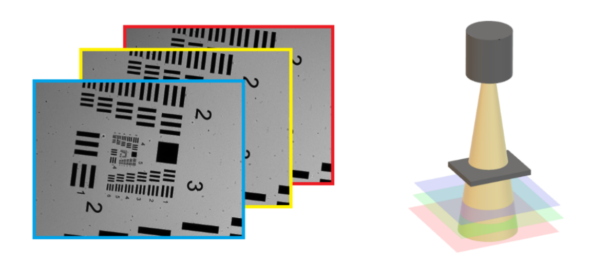
In contrast to multi-height phase retrieval methods, the multi-wavelength approach hinges on capturing images of the same object illuminated by different wavelengths. While the reconstruction distance for a hologram acquired at one wavelength remains fixed, holograms obtained at other wavelengths can be reconstructed as if they were at a proportionately larger or smaller depth (Figure 2).

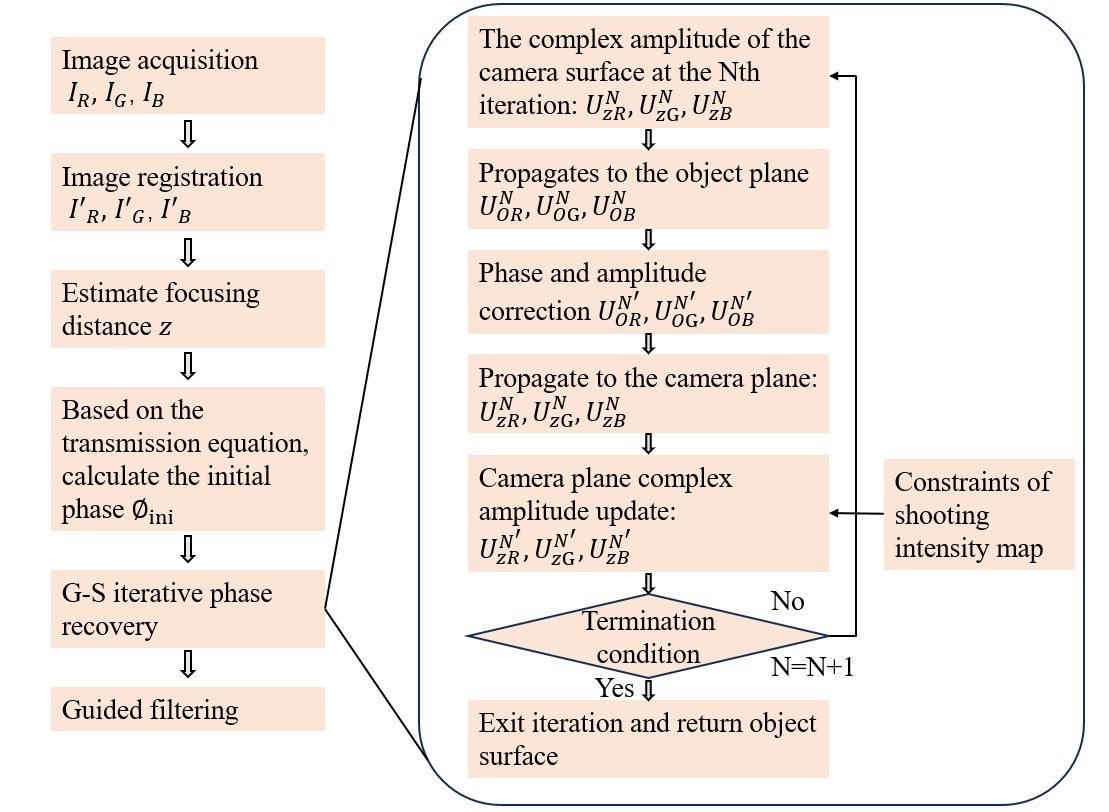
As shown in Figure 3, the process of phase recovering separate to 6 main steps:

1. Image Acquisition: Multiple holograms of the object are captured at different wavelengths of illumination, typically the primary colors of light—red (R), green (G), and blue (B).
2. Image Registration: The images acquired are aligned or registered to ensure they correspond to the same spatial locations.
3. Estimate Focusing Distance ($z$): The reconstruction distances for the holograms are estimated. While the distance for a given wavelength is fixed, other wavelengths can be virtually reconstructed at different depths, simulating a change in focus.
4. Initial Phase Calculation: An initial estimation of the object’s phase profile at one wavelength is made.
5. G-S Iterative Phase Recovery: This iterative process involves the Gerchberg-Saxton algorithm, which is used to recover phase information from intensity images. It alternates between the amplitude captured at one wavelength and the phase estimated at another, propagating the wavefront through virtual planes at different relative depths.
6. Guided Filtering: After the phase recovery, the result might be subjected to guided filtering to refine the outcome.
   To find the reconstruction distance $z$ for each wavelength, the original distance $z_1$ is determined using wavelength $\lambda_1$, the rest $z_i$ corresponding $\lambda_i$ is directly proportional to $z_1$, which could be derived by multiplying the ratio of $\lambda$. So $z_{i}=z_{1} * \lambda_{i} / \lambda_{1}$.

   2.3 Principles of water quality detection by plankton

   Phytoplankton serves as a critical indicator for assessing water quality, as its abundance and species composition are closely linked to the condition of a water body. Variations in phytoplankton populations, either through decline or excessive growth, signal a degradation in water health. Specifically, a surge in phytoplankton, particularly cyanobacteria, and an extended growth period are key indicators of eutrophication in lakes and reservoirs. Pollution directly impacts the species makeup of phytoplankton; while natural water bodies experience seasonal and environmental shifts in algal species composition, these changes are predictable. However, in polluted waters, the alterations in phytoplankton communities due to contaminants are irregular. Golden algae, which are particularly sensitive to environmental shifts, preferring cooler temperatures, low organic content, and high water clarity, demonstrate the most noticeable changes in polluted environments.

In this experiment, in order to estimate the number of plankton in a large volume of water, which could be used to estimate the density of plankton in the whole water body, the water sample should first be concentrated for more efficient estimation. There are several steps in the concentration process.

1. Collect water sample from the top of the water body with volume V(L)
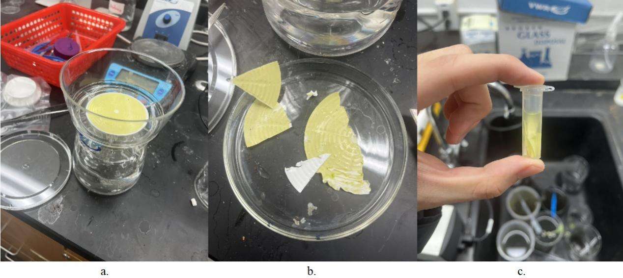
2. Pass the water sample through Bottle Top Filtration Unit with 45 PES filter membrane (Figure 4a)
3. Carefully take off the membrane from the bottle
4. Take 1/6 of the membrane and cut into small pieces (Figure 4b)
5. Add 2 ml of DI water to a microcentrifuge tube
6. Put the pieces of the membrane into the tube
7. Put the tube on the vortex mixer for 1 minute (Figure 4c)
8. Extract 50 of the concentrated water sample and put it on the slide, then put the coverside on

The overall water sample plankton density C (cells/L) after counting the number of plankton in the slide n can be calculated with.
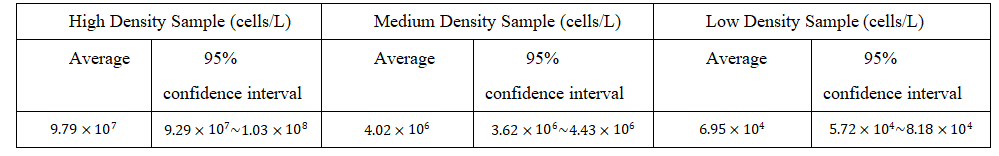
Based on a previous experiment by the Ministry of Ecology and Environment of the People’s Republic of China [22], the following chart is used as a reference.