Project Introduction

About this project

This project introduces a new way to check water health by looking closely at tiny water creatures called plankton. With more pollution due to factories and cities, it’s getting harder to find clean water. Traditional methods to study water are slow. This project uses advanced technology to quickly and accurately study plankton, which helps us understand the quality of water. This method is faster, cheaper, and can spot very tiny details in plankton, making it a great tool for keeping an eye on water health.

1. Introduction

Water covers most of the Earth but is not always easy to use because of pollution. This project focuses on studying small water creatures, plankton, to learn about water quality. Normally, checking water involves a lot of steps and waiting. But with new technologies like digital holographic microscopy, we can get faster and clearer pictures of plankton, helping us understand water quality better and quicker.

2. Basic Principles

2.1 Lens-Free On-Chip Holography

This simple method captures detailed images of plankton using light patterns. It doesn’t need complicated setups like traditional microscopes but still gives us very clear pictures. This helps us see the tiny details of plankton easily.

2.2 Multi-Wavelength-Based Phase Recovery

By taking pictures at different light colors, this method lets us see plankton in even more detail. It uses special algorithms to make images clearer, allowing us to identify small plankton features important for water quality.

2.3 Detection of Water Quality Through Plankton

Plankton changes tell us a lot about water health. This system uses advanced imaging to quickly spot these changes, making it easier to know if the water is clean or polluted.

3. System Design and Construction

3.1 Light Path System Design

The system uses special LED lights and filters to shine different light colors on plankton and captures these images with a camera sensor. This helps get a detailed look at plankton under various light conditions.

3.2 Hardware and Circuit Design

The setup includes several parts controlled by a computer unit, making it easy to switch between different lighting conditions. This simplicity makes it possible to capture high-quality images of plankton for analysis.

3.3 3D Printing and Prototype Building

Using 3D printing, the system’s parts are made precisely and affordably. This approach makes the tool more accessible for monitoring water quality everywhere.

4. Experimentation and Results

The project tested the system with plankton samples and water from different places. Advanced image techniques were used to separate and count plankton in the images, showing the system’s accuracy in spotting water quality changes through detailed plankton analysis.

5. Conclusion

The 3D Digital Holographic Microscopy Water Quality Detection System is a big step forward in monitoring water health. It’s quick, accurate, and affordable, making it easier to check water quality and protect our water resources. Future improvements could include using artificial intelligence to make the system even better at identifying and counting plankton.

Abstract

Water is essential for life but getting clean water is a challenge in many places due to pollution and how water is spread out across the Earth. This study looks at how important it is to check the quality of water, especially with more factories and cities growing. We focus on plankton, tiny water organisms that can tell us a lot about water’s health. When water gets polluted, the type and amount of plankton change, which is a warning sign of poor water quality. Traditional ways of studying plankton involve collecting water samples and analyzing them in labs, which takes a lot of time and can delay getting important information. To make this process faster and more accurate, we use new technologies like digital holographic microscopy (DHM) and lensless digital holographic microscopy (LDHM). These methods allow us to see plankton in great detail and quickly understand water quality.
We explain how we create and analyze images of plankton without using traditional lenses, using light and computers to capture and study these images in detail. This includes using different light wavelengths and advanced computing methods like the Gerchberg-Saxton (G-S) iteration for better image analysis, and techniques like level-set based cell image segmentation for counting and studying plankton cells accurately. Our experiments with these technologies showed that we could see tiny details in plankton, as small as 2.46 micrometers, which is almost as good as the best our equipment can do. This proves that our approach is effective for quickly checking water quality by looking at plankton.
By introducing these new technologies, we provide a faster and cheaper way to monitor water quality, which could help in understanding and protecting aquatic environments better. This research offers a new solution for quickly finding out about water quality through detailed study of plankton, showing a way forward for environmental monitoring.

Introduction

Water, covering two-thirds of the earth’s surface and permanently inundating nearly 4% of the global land mass, is a ubiquitous element. It undergoes a continuous cycle within the hydrosphere, evaporating from the earth’s surface, condensing in the atmosphere, and returning as liquid water. Despite its abundance, water scarcity is a common issue, particularly in regions with uneven distribution. While some places are well-watered, others face shortages, exacerbated by the increasing global population. Although the earth will not run out of water, variations in water quality persist. The majority of the earth’s water is too saline for human use, and pollution from human activities has further degraded the quality of fresh water, diminishing its utility. Even though evaporation serves as a natural water purification process, salts and pollutants left behind continue to contaminate the returning rainwater. Life in all its forms relies on water, making it a vital resource with complexities and challenges that must be addressed [1].
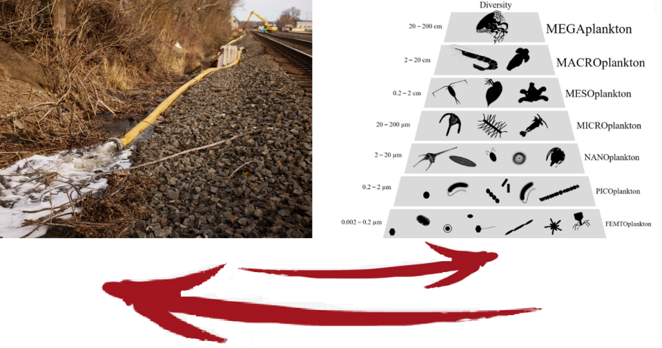
However, with the continuous advancement of industrialization and urbanization, limited water resources is also facing an increasingly serious risk of pollution. For example, on February 3, 2023, a train derailment in Ohio released toxic chemicals into the environment, causing significant water contamination for local residents. Therefore, the detection of water quality has become particularly important. The interconnectedness between the living water environment’s quality and underwater plankton is significant. Stable physiological characteristics, species, and numbers are exhibited by indigenous plankton in various waters. Swift responses to changes in the water body are observed in these organisms. When the water quality experiences pollution to different degrees, variations in plankton species occur due to differing bacterial densities in the water. Optimal water quality is distinguished by moderate pH values, high oxygen content, and low bacterial and microorganism content. In such conditions, higher oval algae, diatoms with columns, and corresponding zooplankton can thrive. Conversely, poor water quality accommodates organisms like sandshell worms, cyclopia, and algae-tolerant strong plankton. Severe water pollution results in high bacterial density, posing a challenge to the survival of most plankton. Only species with stronger pollution tolerance, such as nudibranchs, cyanobacteria, and caecilian earthworms, can endure. Therefore, examining underwater plankton species and quantity allows one to gather information about water quality and its trends, either directly or indirectly.
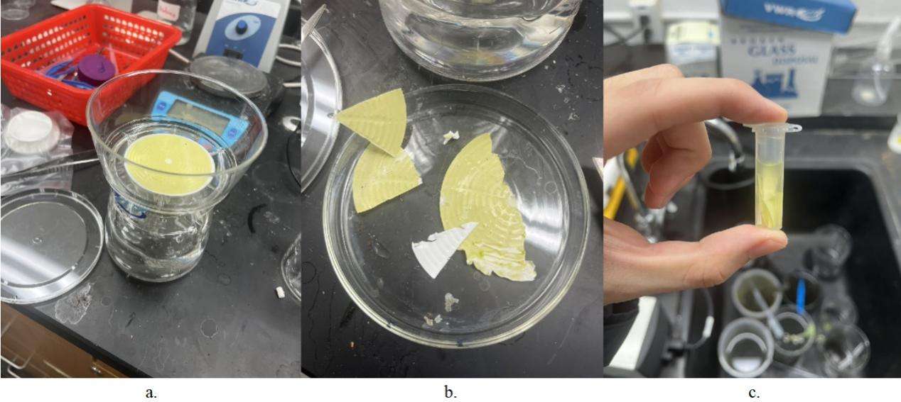
Observation forms the basis for many existing techniques in detecting underwater plankton. Initially, underwater plankton observation relies on a sampling approach. This involved using a sample collector or trawl at a specified water sampling site, and then transporting the sample to the laboratory. Subsequently, the sample underwent a certain degree of treatment, was fixed, and was preserved into observable slide samples. Finally, a laboratory microscope was employed for observation and identification. While sampling observation yields relatively abundant underwater plankton morphology data and reduces identification errors, it comes with notable drawbacks. The process of sampling, transporting to the laboratory, and studying the experimental results introduces significant delays, hindering the timely acquisition of large-scale experimental data for monitoring water quality pollution conditions. Therefore, the traditional sampling-based observation method falls short of meeting the current demands of underwater plankton research and development. To address this, the study of obtaining effective underwater plankton data on a large scale, both temporally and spatially, through relatively simple operations has become a crucial research focus. As multidisciplinary research gains momentum, researchers are increasingly exploring detection methods and tools from other disciplines. Techniques and tools from diverse fields, including biology, acoustics, optics, and electronics, have garnered attention and been integrated into underwater plankton detection research. One such noteworthy approach is the optical detection-based digital holographic imaging method, which stands out for its accuracy, comprehensive experimental data, and effective visualization of results, attracting the interest of experts and scholars with its broad research outcomes and application scope.

Figure 1 Schematic diagram of sewage environment monitoring based on plankton

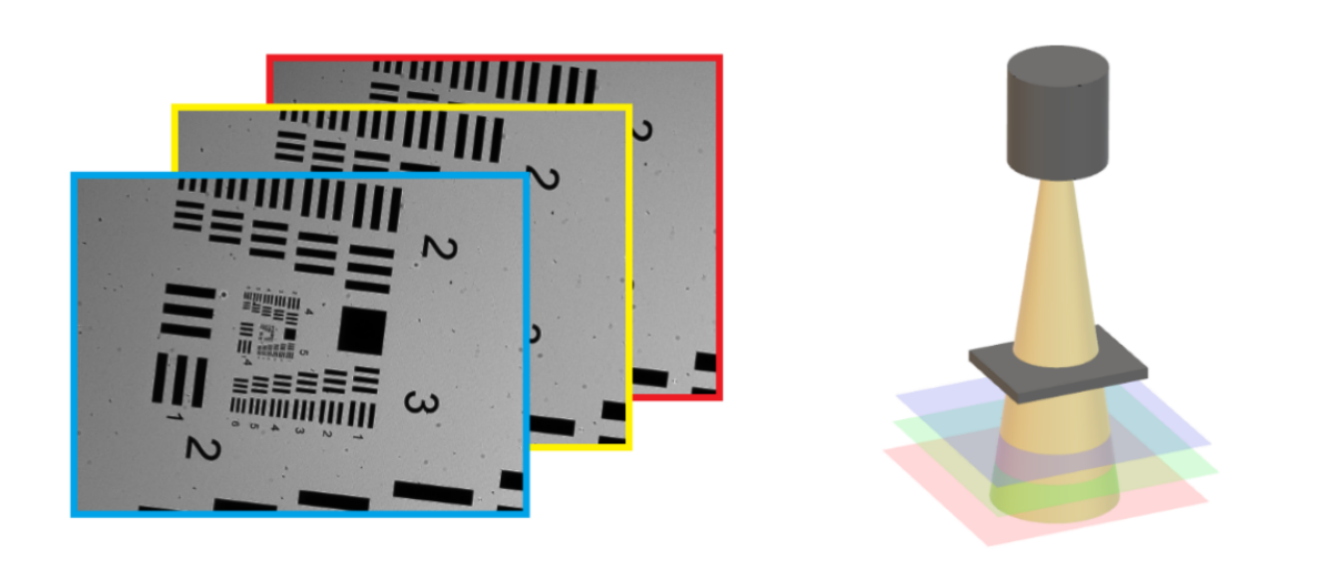
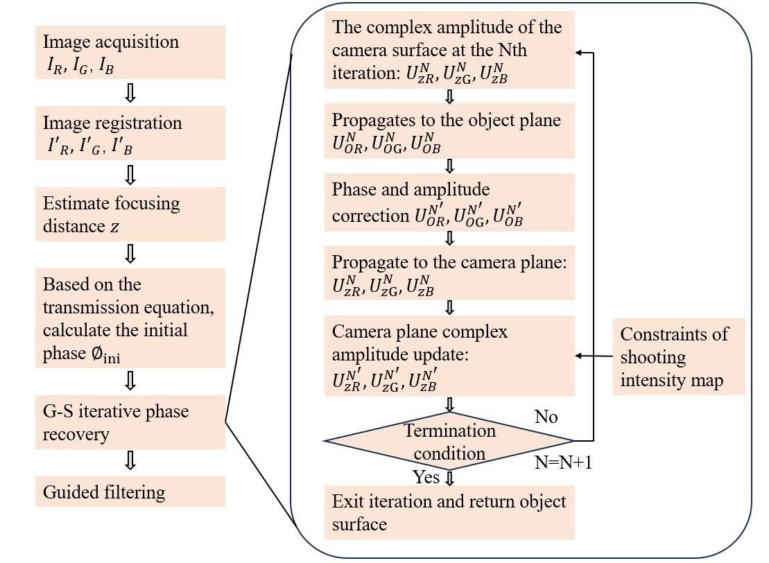
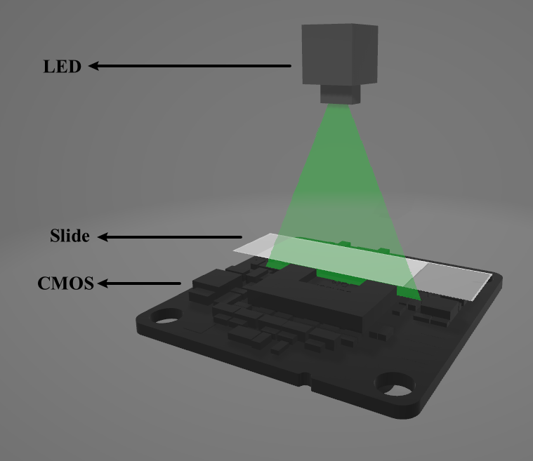
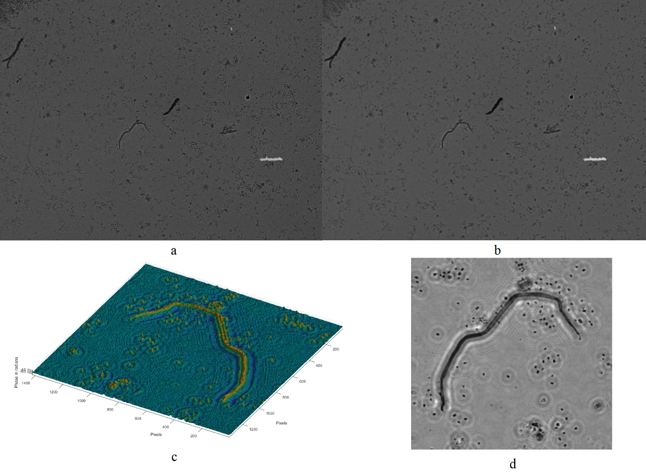
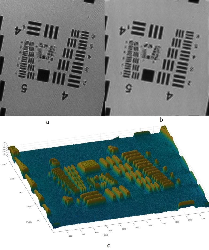
Digital holographic microscopy (DHM) [2] is a widely adopted technique that enables the recording and reconstruction (via the digital holographic principle [3]) of an optical field modulated by various factors such as scattering, refraction, absorption, and reflection from a biomedical [4] or technical micro-object. Hologram demodulation techniques, including Fourier Transform [5], spatial carrier phase shifting [6], or Hilbert Transform [7], along with more precise multi-frame techniques like temporal phase shifting, can provide complex data at the registration plane. The reconstructed complex data contains information about amplitude (absorptive features) and phase (refractive features), which is crucial for label-free quantitative imaging. Over the past two decades, quantitative phase imaging has emerged as a leading framework for label-free live bio-specimen examination [8]. Post-reconstruction, numerical propagation of the optical field to the focus plane is achievable, for instance, using the angular spectrum (AS) method [9], especially when the hologram was captured outside the focus plane. The determination of the focus plane often involves automatic methods like autofocusing approaches [10], now also integrated into deep learning frameworks [11]. Quantitative phase microscopes following DHM principles, as well as traditional bright-field microscopes, are typically bulky with multiple optical elements. In contrast, lensless digital holographic microscopy (LDHM) [12], based on Gabor in-line holography [13], consists of a light source, a CCD camera, and a sample placed between them, preferably near the CCD matrix [14]. This configuration ensures a large field of view (FOV) primarily dependent on the size of the CCD matrix. Resolution in LDHM is mainly limited by the pixel size, requiring it to be small enough to capture dense Gabor holographic fringes without optical magnification [15]. The total number of pixels sampling the hologram is crucial for information bandwidth and resolution.
The recent advancement of lensless imaging owes much to the mass production of affordable digital image sensors with small pixel sizes and high pixel counts [16, 17], alongside improvements in computing power and reconstruction algorithms for processing captured diffraction patterns. Compared to conventional lens-based microscopy, lensless approaches offer key advantages, including a large space–bandwidth product, cost-effectiveness, portability, and depth-resolved three-dimensional imaging. These advantages make lensless imaging particularly suitable for analysis applications requiring extensive statistics, such as cytometry for “needle-in-a-haystack” diagnostic tasks like the Papanicolaou smear test for cervical cancer [18] and blood smear inspection for malaria diagnosis [19]. Lensless imaging is well-suited for studies demanding statistically significant estimates based on limited samples, as seen in the examination of thousands of sperm trajectories to identify rare types of motion [20] and the performance of a complete blood count [21]. Applications with varying number densities, such as air and water quality tests, benefit from lensless imaging’s large space–bandwidth product and depth of field. Lensless imaging is also an excellent choice for point-of-care and global health applications, where compact, portable, cost-effective, and widely distributed devices and approaches are essential. Unlike traditional microscopy, lensless imaging doesn’t require expensive precision microscope objective lenses and light sources. In many instances, individual light-emitting diodes suffice for illumination, and the most expensive component is the image sensor, which can be as low as a few tens of dollars due to mass-produced complementary metal-oxide-semiconductor image sensors for mobile phones [16, 17].

Basic Principles

2.1 Basic principles of lens-free on-chip holography

Lens-free on-chip holography, an in-line digital holographic imaging technique, is introduced with a rearranged sequence of principles for basic recording and numerical reconstruction. The formation of the hologram H(x, y) occurs when a light source with sufficient spatial and temporal coherence illuminates the sample. This hologram is a result of the interference between the scattered light O(x, y) on the sample and the unscattered background light R(x, y). The expression for the hologram is given as:

where r(x, y) and o(x, y) represent the amplitude information of the reference and object lights, and φ(x, y) is the phase information of the object light wave. The light intensity and phase information of the object light wave are obtained using the angular spectrum algorithm, expressed as:

where $F$ and $ F^{-1} $ denote the Fourier transform and the inverse Fourier transform, respectively. G(fx, fy, z) is the optical transfer function in the frequency domain, λ is the wavelength of the light source, and $z$ is the distance from the sample to the sensor plane. In lens-free on-chip microscopy, the small distance ($z$ « $z_2$) between the sample and the sensor is crucial to expanding the field of view and improving resolution, typically ranging from 400 to 1,000 μm. Without a microscope objective, it is necessary to propagate the hologram back to the focal plane. The distance between the sample and the sensor is determined by the autofocusing algorithm in actual operation, resulting in a maximum field of view similar to the image sensor’s working area and a maximum image resolution approximating the sensor’s resolution.
However, the resolution of lens-free on-chip holography is limited by the pixel size of the sensor. To overcome this limitation, reconstruction based on multiple wavelengths is proposed as an effective super-resolution method, capable of removing twin-image simultaneously.

2.2 Multi-wavelength-based phase recovery algorithm

In contrast to multi-height phase retrieval methods, the multi-wavelength approach hinges on capturing images of the same object illuminated by different wavelengths. While the reconstruction distance for a hologram acquired at one wavelength remains fixed, holograms obtained at other wavelengths can be reconstructed as if they were at a proportionately larger or smaller depth (Figure 2).

Figure 2  Schematic diagram of multi-wavelength lighting
Figure 3  Multi-wavelength phase recovery algorithm flow chart

As shown in Figure 3, the process of phase recovering separate to 6 main steps:

  1. Image Acquisition: Multiple holograms of the object are captured at different wavelengths of illumination, typically the primary colors of light—red (R), green (G), and blue (B).
  2. Image Registration: The images acquired are aligned or registered to ensure they correspond to the same spatial locations.
  3. Estimate Focusing Distance ($z$): The reconstruction distances for the holograms are estimated. While the distance for a given wavelength is fixed, other wavelengths can be virtually reconstructed at different depths, simulating a change in focus.
  4. Initial Phase Calculation: An initial estimation of the object’s phase profile at one wavelength is made.
  5. G-S Iterative Phase Recovery: This iterative process involves the Gerchberg-Saxton algorithm, which is used to recover phase information from intensity images. It alternates between the amplitude captured at one wavelength and the phase estimated at another, propagating the wavefront through virtual planes at different relative depths.
  6. Guided Filtering: After the phase recovery, the result might be subjected to guided filtering to refine the outcome.
    To find the reconstruction distance $z$ for each wavelength, the original distance $z_1$ is determined using wavelength $\lambda_1$, the rest $z_i$ corresponding $\lambda_i$ is directly proportional to $z_1$, which could be derived by multiplying the ratio of $\lambda$. So $z_{i}=z_{1} * \lambda_{i} / \lambda_{1}$.

    2.3 Principles of water quality detection by plankton

    Phytoplankton serves as a critical indicator for assessing water quality, as its abundance and species composition are closely linked to the condition of a water body. Variations in phytoplankton populations, either through decline or excessive growth, signal a degradation in water health. Specifically, a surge in phytoplankton, particularly cyanobacteria, and an extended growth period are key indicators of eutrophication in lakes and reservoirs. Pollution directly impacts the species makeup of phytoplankton; while natural water bodies experience seasonal and environmental shifts in algal species composition, these changes are predictable. However, in polluted waters, the alterations in phytoplankton communities due to contaminants are irregular. Golden algae, which are particularly sensitive to environmental shifts, preferring cooler temperatures, low organic content, and high water clarity, demonstrate the most noticeable changes in polluted environments.

Figure 4   Physical picture of plankton laboratory processing a: water filtering, b: filter paper cutting, c: filter paper redissolution

In this experiment, in order to estimate the number of plankton in a large volume of water, which could be used to estimate the density of plankton in the whole water body, the water sample should first be concentrated for more efficient estimation. There are several steps in the concentration process.

  1. Collect water sample from the top of the water body with volume V(L)
  2. Pass the water sample through Bottle Top Filtration Unit with 45 PES filter membrane (Figure 4a)
  3. Carefully take off the membrane from the bottle
  4. Take 1/6 of the membrane and cut into small pieces (Figure 4b)
  5. Add 2 ml of DI water to a microcentrifuge tube
  6. Put the pieces of the membrane into the tube
  7. Put the tube on the vortex mixer for 1 minute (Figure 4c)
  8. Extract 50 of the concentrated water sample and put it on the slide, then put the coverside on

The overall water sample plankton density C (cells/L) after counting the number of plankton in the slide n can be calculated with.
Based on a previous experiment by the Ministry of Ecology and Environment of the People’s Republic of China [22], the following chart is used as a reference.
Table 1

Plankton detection system design and construction

3.1 Overall light path system design

The diagram below illustrates the light path of the digital microscope, starting with an LED that provides a stable source of light. This light illuminates the specimen mounted on a slide, and the interaction between the light and the sample is captured by the CMOS.

Figure 5   Schematic diagram of system optical path structure

In order to have multi-wavelength light, there are several ways to complete this system. One is to let the LED become multi-wavelength so that it can emit different light on a different wavelength. Another is to add a multiple-filter control system, including a plate holding filter of different wavelengths and a servo. By turning the plate so that light passes through different filters, the different wavelengths of light can be achieved.

3.2 Hardware and circuit design

Figure 6   Schematic diagram of system hardware path structure

The whole system contains a total of six components without the Micro Control Unit (MCU), mainly including the outer shell, slide holder, CMOS, servo with filter, and LED. The adjustable holder (2) is an instrument that can change the height of the plate precisely. To switch between different filters, a servo is used to rotate the plate to choose the filter. The LED light shell is designed to hold one white LED with an aluminum base. To connect the system with the MCU, the positive and negative wires of the servo and the positive wire of the LED are directly connected to the 5V and GND ports in the MCU. The signal wire of the servo is connected to the analog output port of the MCU, and the negative wire of the LED is connected to the digital output port of the MCU. By programming the MCU to control the related output in different ports, the LED switch and the position of the servo can be controlled. The output wire of the CMOS can be directly connected to the computer to record the picture captured, or if the MCU is Raspberry Pi or similar hardware that has USB-A and wireless communication equipment, the CMOS could also directly connect to the MCU and wirelessly read data on a computer for later analysis.

3.3 3D printing and prototype building

For the outer shell, slide holder, and filter plate, the 3D printing material is photosensitive resin using the SLA process. An SG90 servo is used in this system because of its small size. A 5050 LED is used since it can separately control all three RGB values, and the distance between three small LEDs is in an acceptable range. A narrowband filter is used since a limited wavelength is required for the phase retrieving process to be accurate. The half-band width of the three filters is 20nm, and the wavelength for the three filters is 650nm, 532nm, and 450nm. The CMOS type is Basler dart daA2500-14um (No-Mount), with resolution (H x V) 2592 px × 1944 px, pixel Size (H x V) 2.2 μm × 2.2 μm, frame rate 14 fps, and mono color.
In order to assemble the system, the slide holder should be inserted into the supporting component in the middle bottom hole and fixed with glue. The CMOS and its supporting components should be fixed with a screw and nut. The wire should be appropriately carried out by drilling holes in the supporting component. After making sure the output port of the CMOS is exposed and gluing the front board of the supporting component on, assemble the filter plate with all three filters, and then attach the filter plate to the servo. Then, screw the servo and its supporting component to the outer shell, and make sure all wires are correctly connected as stated in the “Hardware and circuit design” section. Finally, assemble the outer shell with the supporting component, and do the first test of the system.

Experiment

4.1Plankton slide sample testing

In order to test the performance of the system, the sample slide of paramecium is used. After taking the background image (which follows the same process but without the slide on), there are several steps to follow:

  1. Fix the slide on the slide holder, and connect the camera to the receiver device.
  2. Adjust the height of the slide holder to minimize the distance between the slide and the CMOS.
  3. Open one of the RGB LEDs or turn the filter plate to one of the RGB filters.
  4. Record the picture in the receiver (computer or MCU).
  5. Repeat steps 3 and 4 to take pictures under all the lights.

After taking the photo, three background images and three object images are processed as in Figure 4. The image before and after processing is shown in Figure 7.
Figure 10a provides the original image taken under green light of 525μm. As shown in Figure 10b, the clarity of the image greatly improved. Figure 7c shows the processed image of one specific paramecium. The 3D shape of one specific paramecium can be derived as shown in Figure 7d.

Figure 7   Observation results of paramecium slide sample a: hologram b: light intensity diagram after processing c: light intensity of a single paramecium d: 3d image of a single paramecium

4.2Water quality sample collection

After making the concentrated water sample slide using the process illustrated in section 2.3, the sample can be recorded using the process illustrated in 4.1. The number of cells in the processed image can be calculated using level-set based cell image segmentation.
Level-set based cell image segmentation is an advanced image processing method for recognizing and segmenting cells from complex backgrounds. This technique is very important in biomedical imaging analysis, especially in cases where individual cells need to be accurately identified and quantified. The following is the basic process of level set based cell segmentation technique:

  1. Image Acquisition and Preprocessing: after processing to obtain images of the observed microorganisms, the images need to be pre-processed. This includes steps such as denoising, contrast adjustment, grayscaling etc.
  2. Level Set Function: The level set method relies on a mathematical representation called the level set function, which is used to define the foreground (e.g., cells) and background in the image. The level set function is evolved through a mathematical formulation (usually a partial differential equation). This process causes the contours of the level set to gradually move towards the cell boundaries.
  3. Segmenting the Cell: When the level set function is stable, i.e., the contour no longer changes significantly, it is considered to be close to or at the actual boundary of the cell. At this point, this contour can be used to segment out the cells in the image.
  4. Post-processing: The segmented result may require some post-processing, such as removing regions that are too small (which may be noise), or merging regions that are very close together (which may be different parts of the same cell).

Figure 8   Cell identification technology

The number of cells calculated by the above method is only the number of cells inside the view of the CMOS. In order to estimate the complete number of cells on the slide , the ratio of the CMOS area and slide area is used for estimation with the formula ${n_t} = {n_c}*{S_s}/{S_c}$

Figure 9   Water sample observation results a: hologram b: light intensity diagram after processing c: 3D image of a part of sample d: light intensity of a part of sample

In Figure 9, the water sample from a pond in the Princeton area is processed using the above procedure. Figure 9a shows the original image of the concentrated water sample, and Figure 9b is the image after phase retrieval. Figure 9d shows the phase retrieved image of a small part of the image, and Figure 9c shows the 3d shape of the image.

4.3 Overall analysis

Figure 10   Resolution board sample observations a: hologram b: light intensity diagram after processing c: 3D image

In order to get a more systematic evaluation of the system, the USAF1951 resolution board is used. As shown in Figure 10, Figure 10a is the original image under green light of 525μm, and Figure 10b is the processed image. The system can capture at most group 7 element 5 clearly, which is 2.46μm. In this test case, the CMOS we tested has a pixel size of 2.2μm by 2.2μm, so the system is approaching the theory limit resolution of the hardware.

Conclusion

Our study into digital holographic microscopy (DHM) and lensless digital holographic microscopy (LDHM) as tools for assessing water quality through plankton analysis marks a significant step towards innovative environmental monitoring methods. Plankton analysis stands out as a key indicator of water health, revealing that rapid and accurate detection of water quality changes is achievable. This approach significantly outperforms traditional methods, which are slower and may not keep pace with the swift changes in water bodies caused by pollution. The benefits of utilizing DHM and LDHM are manifold. These technologies enable quick observation and analysis of plankton, dramatically reducing the time needed to evaluate water quality. Through capturing high-detail plankton images and applying sophisticated image analysis algorithms like the G-S iteration and level-set based cell image segmentation, we manage to precisely measure and identify plankton species and quantities. Testing with the USAF1951 resolution board confirmed our system’s capability to distinguish features as small as 2.46μm, proving its high resolution and accuracy. Moreover, these optical techniques streamline the necessary equipment for plankton observation, making the process both more accessible and cost-effective. This opens up water quality monitoring to a broader audience, allowing more communities and researchers to perform their own assessments and make well-informed decisions on water management and conservation.
Looking ahead, there’s potential to build upon our findings. Future research might delve into incorporating artificial intelligence and machine learning to automate plankton identification and counting, which could further expedite and refine analysis accuracy. Expanding the plankton image database to include various conditions could enhance system sensitivity to different pollution types. Additionally, improving the portability and field-readiness of the equipment could extend its usability across varied environmental settings.
In closing, our investigation presents a solid proof of concept for applying advanced optical methods in water quality monitoring through plankton analysis. Advancing this groundwork, future endeavors can augment the efficiency, reach, and impact of water quality monitoring efforts, contributing significantly to the worldwide initiative to safeguard our essential water resources.

References

  1. Boyd, C. (2012). Water quality. Aquaculture: farming aquatic animals and plants. Wiley-Blackwell, Oxford, 52-83.
  2. M.K. Kim, Digital Holographic Microscopy (Springer, 2011).
  3. U. Schnars and W. Jueptner, Digital Holography (Springer, 2005).
  4. B. Kemper and G. von Bally, “Digital holographic microscopy for live cell applications and technical inspection,” Appl. Opt. 47(4), A52–A61 (2008).
  5. M. Takeda, H. Ina, and S. Kobayashi, “Fourier-transform method of fringe-pattern analysis for computer-based topography and interferometry,” J. Opt. Soc. Am. 72(1), 156–160 (1982).
  6. M. Pirga and M. Kujawinska, “Two directional spatial-carrier phase-shifting method for analysis of crossed and closed fringe patterns,” Opt. Eng. 34(8), 2459 (1995).
  7. T. Ikeda, G. Popescu, R. Dasari, and M. Feld, “Hilbert phase microscopy for investigating fast dynamics in transparent systems,” Opt. Lett. 30(10), 1165–1167 (2005).
  8. Y. Park, C. Depeursinge, and G. Popescu, “Quantitative phase imaging in biomedicine,” Nat. Photonics 12(10), 578–589 (2018).
  9. T. Kozacki and K. Falaggis, “Angular spectrum-based wave-propagation method with compact space bandwidth for large propagation distances,” Opt. Lett. 40(14), 3420–3423 (2015).
  10. Y. Zhang, H. Wang, Y. Wu, M. Tamamitsu, and A. Ozcan, “Edge sparsity criterion for robust holographic autofocusing,” Opt. Lett. 42(19), 3824–3827 (2017).
  11. Y. Wu, Y. Rivenson, Y. Zhang, Z. Wei, H. Günaydin, X. Lin, and A. Ozcan, “Extended depth-of-field in holographic imaging using deep-learning-based autofocusing and phase recovery,” Optica 5(6), 704–710 (2018).
  12. A. Ozcan and E. McLeod, “Lensless Imaging and Sensing,” Annu. Rev. Biomed. Eng. 18(1), 77–102 (2016).
  13. E. McLeod and A. Ozcan, “Unconventional methods of imaging: computational microscopy and compact implementations,” Rep. Prog. Phys. 79(7), 076001 (2016).
  14. D. Gabor, “A New Microscopic Principle,” Nature 161(4098), 777–778 (1948).
  15. T. Agbana, H. Gong, A. Amoah, V. Bezzubik, M. Verhaegen, and G. Vdovin, “Aliasing, coherence, and resolution in a lensless holographic microscope,” Opt. Lett. 42(12), 2271–2274 (2017).
  16. Vashist SK, Mudanyali O, Schneider EM, Zengerle R, Ozcan A. 2013. Cellphone-based devices for bioanalytical sciences. Anal. Bioanal. Chem. 406:3263–77
  17. Ozcan A. 2014. Mobile phones democratize and cultivate next-generation imaging, diagnostics and measurement tools. Lab Chip 14:3187–94
  18. Greenbaum A, Ozcan A. 2012. Maskless imaging of dense samples using pixel super-resolution based multi-height lensfree on-chip microscopy. Opt. Expr. 20:3129–43
  19. Bishara W, Sikora U, Mudanyali O, Su T-W, Yaglidere O, et al. 2011. Handheld, lensless microscope identifies malaria parasites. SPIE Newsroom, Aug. 5. http://spie.org/x51571.xml
  20. Su T-W, Choi I, Feng J, Huang K, McLeod E, Ozcan A. 2013. Sperm trajectories form chiral ribbons. Sci. Rep. 3:1664
  21. Seo S, Isikman SO, Sencan I, Mudanyali O, Su T-W, et al. 2010. High-throughput lens-free blood analysis on a chip. Anal. Chem. 82:4621–27
  22. Ministry of Ecology and Environment of the People’s Republic of China. (2021). Water quality—Determination of Phytoplankton—Membrane filtration method (Report No. HJ 1216-2021). Ministry of Ecology and Environment of the People’s Republic of China https://big5.mee.gov.cn/gate/big5/www.mee.gov.cn/xxgk2018/xxgk/xxgk06/202009/W020200930591312856871.pdf

3D File and Example Code

Example code of single wavelength reconstruction (to estimate the distance):

1
2
3
4
5
6
7
8
9
10
11
12
13
14
15
16
17
18
19
20
21
22
23
24
25
26
27
28
29
30
31
32
33
34
35
36
37
38
39
40
41
42
43
44
45
46
47
48
49
50
51
52
53
54
55
56
57
58
59
60
61
62
63
64
65
66
67
68
69
clc;
close all;
clear;
set(0,'defaultfigurecolor','w');%background color white
I=imread('G.tiff'); %Hologram
I0=imread('BG.tiff'); %Background
I = double(I);
I0 = double(I0);
[N,M]=size(I);
figure(1);imshow(I,[]);title('Original Hologram');
I1=I;
Rect=round(getrect);
Xmin=max(Rect(1),1);
Ymin=max(Rect(2),1);
Xmax=(Rect(1)+Rect(3));
Ymax=(Rect(2)+Rect(4));
hold on;
plot([Xmin Xmax Xmax Xmin Xmin],[Ymin Ymin Ymax Ymax Ymin],'r');
hold off;
I1=I(Ymin:Ymax,Xmin:Xmax);
[N,M]=size(I1);
I0=I0(Ymin:Ymax,Xmin:Xmax);
lamda=525*10^-9;
for kk = 0:1
%d=(0.6+0.4*kk/10)*10^-3;
d=0.88*10^-3;%Estimated Distance
k=1.5*pi/lamda;
dx=2.2*10^-6;
dy=2.2*10^-6;
dfx=1/(M*dx);
dfy=1/(N*dy);
fx=ones(N,1)*(-M/2:M/2-1)*dfx;
fy=(ones(M,1)*(-N/2:N/2-1)*dfy)';
hol_fft111=fftshift(fft2(I1));
hol_fft=fftshift(fft2(I1));
obj_fft=hol_fft.*exp(1i*k*(-d)*sqrt(1-lamda^2*(fx.^2+fy.^2)));
obj=ifft2(ifftshift( obj_fft));
amp_obj=abs(obj);
obj_phase=angle(obj);
figure(kk+3);imshow( amp_obj,[]);title('Intensity');
%figure(3);imshow( amp_obj,[]);title('Intensity');
%figure(4);imshow( obj_phase,[]);title('Phase');

end
phase1=obj_phase;
AAA=I1./I0;
amp_hol=I1./I0;
hol_phase=0;
for kk = 1:10
hol=amp_hol.*exp(1i.*hol_phase);
hol_fft=fftshift(fft2(hol));
obj_fft=hol_fft.*exp(1i*k*(-d)*sqrt(1-lamda^2*(fx.^2+fy.^2)));
obj=ifft2(ifftshift( obj_fft));
amp_obj=abs(obj);
obj_phase=angle(obj);
%obj_phase(amp_obj>0.58)=-obj_phase(amp_obj>0.58);
amp_obj(amp_obj>0.88)=1;
%amp_obj=kkk;
obj_1=amp_obj.*exp(1i.*obj_phase);
obj_1_fft=fftshift(fft2(obj_1));
hol_fft=obj_1_fft.*exp(1i*k*(d)*sqrt(1-lamda^2*(fx.^2+fy.^2)));
hol=ifft2(ifftshift( hol_fft));
hol_phase=angle(hol);
end
figure(5);imshow(abs(obj),[]);title('Intensity');
figure(6);imshow(angle(obj),[]);title('Phase');
I=abs(obj);
P=angle(obj);
mesh(P);